
| News and Announcements » |
This tutorial covers how to perform Procrustes Analysis using Qiime to compare beta diversity plots generated by two different mechanisms. Procrustes analysis takes as input two coordinate matrices (in Qiime, these are usually the results of running a principal coordinates analysis on a sample-by-sample distance matrix), and transforms the second coordinate set to minimize the distances between corresponding points. The results can then be visualized using Qiime by running compare_3d_plots.py – both sets of coordinates will be plotted in the resulting figure, with bars connecting the corresponding points from each data set.
For example, Figure 1 is a plot that was generated by comparing two different sets of reads from the same collection of samples. The idea behind this study was to evaluate whether the same beta diversity conclusions would be derived from different read types. Bars connect points from the same sample, where each point represents one read type. Colors, as usual in Qiime 3D plots, indicate sample type (for example, dark blue represents 5 fecal samples). The two read types compared are the 5’ reads and the 3’ reads from a paired-end Illumina run. The results here illustrate that the 3D plot derived from each read type is essentially identical, and the different read types would certainly not lead to different conclusions.
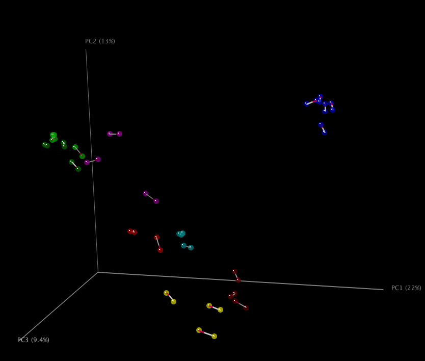
Figure 1: Procrustes comparison of unweighted UniFrac PCoA plots derived from 5’ and 3’ reads from a paired-end Illumina run. A discussion of this analysis can be found in Caporaso et al., PNAS (2010), “Global patterns of 16S rRNA diversity at a depth of millions of sequences per sample”.
To visualize procrustes results on two principal coordinate matrices with overlapping sample IDs, you can run the following command:
transform_coordinate_matrices.py -i pcoa1.txt,pcoa2.txt -o procrustes/
In this example `` pcoa1.txt`` and pcoa2.txt are your two principal coordinate matrices. Note that these are comma-separated with no spaces between them. The output will be two transformed principal coordinate matrices which can be provided to compare_3d_plots.py with the command:
compare_3d_plots.py -i procrustes/pc1_transformed.txt,procrustes/pc2_transformed.txt -m mapping_file.txt -o plots/
The 3D Procrustes plots will be written to plots/.
Transform coordinate matrices also supports generation of monte carlo p-values based on a user-specified number of repetitions. To generate this data, you could modify your transform_coordinate_matrices.py command by appending the -r parameter as:
transform_coordinate_matrices.py -i pcoa1.txt,pcoa2.txt -o procrustes/ -r 1000
This specifies that 1000 repetitions should be run. The output of this analysis will be in the output directory in a file named based on the input files (procrustes/pcoa1_pcoa2__procrustes_results.txt in this example).